
Probability Distributions 101
A (re)primer on basic probably distributions

"You'll never use most of the things you learn in College."
- Olshansky circa 2014
There was a time when I thought that most of what I learnt in College was pointless since it didn't apply to my day-to-day work. However, as time passes, I increasingly reflect on how fortunate I was to be exposed to so many concepts across various fields. Most importantly, it teaches you to think, learn and work, but I'll save the details for another post.
Whenever an opportunity arises to apply something I learnt in school that I don't use frequently, I find myself needing to go back and review the basics, but also take it as an opportunity to truly understand the fundamentals. There is beauty in understanding a subject rather than just submitting an assignment or acing a test.
At work, I recently needed to model a basic probability distribution to determine the values for certain parameters. The tools for the job are taught in an average grade 12 Data Management course, but figuring out which tool to use was the hard part. I came across this simple primer from the University of North Florida, but it wasn't quite what I was looking for, so I embarked on a journey with a few of my good friends: Google, Wikipedia and ChatGPT.
** This is not meant to be an exhaustive "literature review" of all the different probability distributions or concepts. Instead, it is a small opinionated list of concepts I found useful and interesting.
The Basics
Probability: The likelihood of an event occurring.
Probability theory: A branch of mathematics founded on 3 Probability Axioms.
Probability Distribution: A function of random events happening over some sample space.
Random Variable (RV): Variables used to describe the random event. It can be Discrete (e.g. 🎲, 🪙) or Continuous (e.g. ⚖️, 📏).
Probability Mass Function (PMF): Describes the values, and their probabilities, of a Discrete Random Variable.

Fun fact: The probability of a Continous Random Variable (CRV) taking on any exact value is 0.
Probability Density Function (PDF): The density (i.e. the rate of change) of a CRV. This can be used to compute (i.e. integrate) the probability of a CRV being within a certain range.
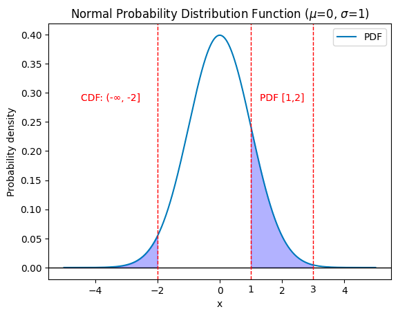
Cumulative Distribution Function (CDF): The probability that a random variable is less than or equal to some value.

Starting off Normal
We can start things off normally with the well-known Gaussian distribution, aka the Normal Distribution, aka the Bell Curve.
={\frac {1}{\sigma {\sqrt {2\pi }}}}e^{-{\frac {1}{2}}\left({\frac {x-\mu }{\sigma }}\right)^{2}}}")
Mean (µ): The average, module and mode of the distribution.
Standard Deviation (σ): A measure of how much the values disperse around the mean.
Euler's Number (e): eiπ + 1 = 0

Gaussian (Normal) Distribution: Probability distribution common in various circumstances (natural phenomena, experiments, finance, etc.). Answers the question: “What percentage of my data is within some variation from the average?”

Bernoulli What?
You may have heard of Bernoulli in various contexts, and it’s because their family was full of renowned academics. They relocated from Antwerp to Basel in 1620, and the rest, as they say, is history. We’ll focus on Jacob Bernoulli’s work, who coined (🥁) the term Bernoulli Trial to describe simple events such as flipping a coin.

Disclaimer: The delineation between Bernoulli X and Binomial X gets a bit blurry in terms of Trials, Processes, Experiments, Distributions, etc. The definitions below should be treated as my best-effort understanding and guiding principle rather than as fact.
Bernoulli Event: An event with two outcomes: success (p) or failure (q=1-p). For example, if we define rolling a 3 as success, then: p=1/6 and q=5/6.
Bernoulli Trial: A single experiment (i.e. an instantiation) of a single Bernoulli Event.
Bernoulli Process: A sequence of (potentially infinite) independent Bernoulli Trials.
** The terms above are used in more theoretical and formal definitions, but we usually encounter the term Binomial in practice.
Bernoulli Distribution: A special case of the Binomial Distribution with exactly one trial (n=1).
Binomial Distribution: A probability distribution of k success in n Bernoulli Trials. Answers the question: “What is the probability of succeeding k times in exactly n independent trials irrespective of order?”
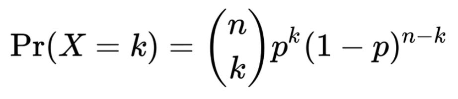
For example, what is the probability of rolling a 3 (p=1/6, q=5/6), 2 times (k=2), given a total of 10 rolls (n=10)? Using the above equation plotted below, we see it’s just under 30%.

Geometric Distribution: Discrete probability distribution that models the number of trials needed to achieve the first success in a sequence of independent Bernoulli trials. Answer the question: “How likely am I to fail k times until I succeed once?”
=(1-p)^{k-1}p}")
For example, if I want to succeed (roll a 3), how likely am I to roll the die 10 times (k=10) before it happens? Using the above equation plotted below, we see it’s just under 2.5%.

Negative Binomial Distribution: A probability distribution of the number of failures, r, to occur until achieving k success. Answers the question: “If I succeed with probability p, what is the likelihood that I’ll fail r times before I succeed k times?”

For example, if I want to succeed (roll a 3) a total of 2 times (n=2), what is the probability of me failing (rolling anything other than a 3) a total of 5 times (r=5) while doing so? Using the above equation plotted below, we see it’s just under 7%.

Something Smells Fishy…
In 1837, more than a hundred years after Jacob Bernoulli first introduced the Bernoulli distribution to the world in 1713, the French mathematician Siméon Denis Poisson learnt to fish and introduced the Poisson distribution. It is a special case of the Bernoulli distribution where the number of trials (n) becomes very large, and the probability of success (p) becomes very small, such that the product (n*p) remains constant.
Poisson Distribution: Probability distribution expressing the likelihood of a given number of events occurring in a fixed interval of time given that these events occur independently and at a constant rate. Answers the question: “Given that this event happens at some frequency, how likely is it that it’ll happen k times within some period of time?”
λ: Average rate of events per unit time; λ = Mean(X) = Variance(X)
r: the rate at which the events happen per unit of time
k: The number of occurrences of the event at hand

={\frac {(rt)^{k}e^{-rt}}{k!}}.}")
For example, what is the probability of 6 (k=6) ducks walking into my house today, given that, on average, 3 ducks (λ=3) walk into my house each day? Looking at the distribution below, we see that the probability is ~5%.

Exponential distribution: Probability distribution modelling the time between events in a Poisson process. Answers the question: “Given that this event happens at some frequency, what is the likelihood that some specific amount of time will pass between two consecutive events?”
λ: Average rate of events per unit time; Mean(X) = 1 / λ; Variance(X) = 1 / λ2
x: The amount of time that will pass between two events
={\begin{cases}\lambda e^{-\lambda x}&x\geq 0,\\0&x<0.\end{cases}}}")
For example, what is the probability of 1 day (x=1) passing between two consecutive ducks walking into my house given that, on average, half a duck walks into my house each day (i.e. 1 duck every 2 days)? Looking at the distribution below, we see that the probability is ~25%.

Story Time
At the age of 5, when my mom was first teaching me about fractions and percentages, the most difficult concept for me to grasp was why percentages were measured on a scale of 0 to 100. A range from 0 to 1 makes sense, a scale of 0 to ∞ could make sense, but 100 felt so random and arbitrary. Why not 1,000%, why not 10,000%? Eventually, I gave up and just accepted it.
According to Wikipedia, it’s because taxes were levied in increments of 1/100 in Ancient Rome, and things just stuck around.

The code for all of these charts was generated with the help of ChatGPT and is available in this GitHub gist for reference.
A friend of mine provided me some deep feedback on this article, so I wanted to share it here publicly for posterity purposes with my updated learnings.
---
> Unfortunately, your "fun fact" isn't entirely true!
> > "Fun fact: The probability of a Continuous Random Variable (CRV) taking on any exact value is 0."
> In a Dirac distribution, P(x) is 0 everywhere except at one location, where the pdf is such that the integral comes out to 1. So P(y) is 1 for that value.
I learnt that the Dirac delta function is used to represent point impulses. It represents an infinitely narrow spike of probability density at a single point (equaling to 1) and is zero everywhere else. It's integral over the entire real line is equal to 1.
> Bernoulli vs Binomial is such an unfortunate linguistic situation. Such similar concepts. Such similar names. One of the names is semantically unrelated to the meaning of the terms. The other maps closely to the meaning, but is more suggestive of the wrong meaning imo. Bernoulli == single coin flip; Binomial == counting heads.
To reiterate the main point here:
* Bernoulli == single coin flip
* Binomial == counting heads
> Further confused by using dice-rolling as an example -- you do it correctly, but it's suggestive of a six-outcome event whereas we're concerned with just 2-outcome events.
* Bernoulli == single die role
* Binomial == counting number of times a 3 is rolled versus other ([1,2,4,5,6])
> Negative Binomial Distribution: that was a new term for me
Glad we're all always learning :)
> Silly section titles 👌
> Duck probabilities
🦆🦆🦆
> It looks like you just read off the Poisson PDF (0.25)
> Instead, you'd need to choose a range (e.g. 1-2 days) and integrate the pdf over this range (or evaluate the cdf at start and end of range, and subtract end-start). As you noted in your fun fact earlier, the probability of it being exactly one day between duck arrivals is 0!
Even though I do have a CDF, I confused myself because of the numbers I selected and how I defined them, so I'm going redefined the problem here.
* What is the event? Let's assume a duck walking into my house is the event.
* Lambda = 0.5 => time between events is "half a day". A duck walks into my house every half a day, on average. Alternatively, two ducks walk into my house every day, on average.
* Question #1: What is the probability of there being a whole day where a duck doesn't walk into my house?
1 - CDF(P(X >= 1)) ~= 1 - 0.9 = 0.1 = 10%
* Question #2: What is the probability of a duck coming into my house in 6 hours or less (i.e. a quarter of a day)?
CDF(P(X <= 0.25)) ~= 0.3 = 30%
* Question #3: What is the probability of 4 ducks walking into my house in 1 day?
It would be the answer to question #2 to the power of 4
> ChatGPT usage.
> Very cool 🙂
🤖 It is my friend, partner, tutor, assistant and so much more 🤖